Category Archives: chart

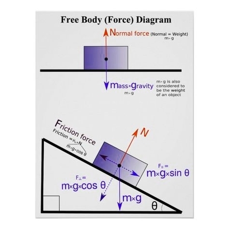
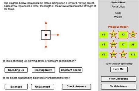
Free body force physics is a branch of physics that deals with the analysis of forces and moments acting on a body in a given situation. A free body diagram (FBD) is a graphical tool that helps to visualize and simplify the problem by showing only the relevant forces and their directions. Here is an example of a free body diagram for a block resting on a ramp:

“`latex
begin{tikzpicture}
% Draw the ramp
draw[thick] (0,0) — (4,2);
draw[dashed] (0,0) — (4,0);
draw[<->] (2,0) arc (0:26.6:2) node[midway,right] {$theta$};
% Draw the block
draw[fill=gray] (2.5,1.25) rectangle (3.5,2.25) node[midway] {$m$};
% Draw the forces
draw[->,red,thick] (3,2.25) — (3,3.25) node[above] {$F_N$};
draw[->,red,thick] (3,1.25) — (3,0.25) node[below] {$mg$};
draw[->,red,thick] (2.5,1.75) — (1.5,1.75) node[left] {$F_f$};
end{tikzpicture}
“`

In this diagram, the block has a mass $m$ and is subject to three forces: the normal force $F_N$, the weight $mg$, and the friction force $F_f$. The angle of the ramp is $theta$. The goal of free body force physics is to find the magnitude and direction of these forces, as well as the acceleration and motion of the block, using Newton’s laws of motion and some basic trigonometry.

One of the main principles of free body force physics is that the net force on a body is equal to its mass times its acceleration, or $sum F = ma$. This means that we can write equations for the horizontal and vertical components of the net

Moore’s Law is an empirical observation that the number of transistors in an integrated circuit (IC) doubles approximately every two years. It is named after Gordon Moore, the co-founder of Fairchild Semiconductor and Intel. Moore’s Law is not a law of physics, but rather an observation and projection of a historical trend. The observation was first made in 1965, when Moore posited a doubling every year in the number of components per integrated circuit, and projected this rate of growth would continue for at least another decade. In 1975, looking forward to the next decade, he revised the forecast to doubling every two years, a compound annual growth rate (CAGR) of 41%. While Moore did not use empirical evidence in forecasting that the historical trend would continue, his prediction has held since 1975 and has since become known as a “law” .

Moore’s Law has been used in the semiconductor industry to guide long-term planning and to set targets for research and development, thus functioning to some extent as a self-fulfilling prophecy. Advancements in digital electronics, such as the reduction in quality-adjusted microprocessor prices, the increase in memory capacity (RAM and flash), the improvement of sensors, and even the number and size of pixels in digital cameras, are strongly linked to Moore’s Law . These ongoing changes in digital electronics have been a driving force of technological and social change, productivity, and economic growth.

However, industry experts have not reached a consensus on exactly when Moore’s Law will cease to apply. Microprocessor architects report that semiconductor advancement has slowed industry-wide since around 2010, slightly below the pace predicted by Moore’s law . The slowing of Moore’s Law has been attributed to several factors, including the increasing difficulty of manufacturing at smaller scales, the increasing cost of research and development, and the physical limitations of the materials used in semiconductor manufacturing .

In conclusion, Moore’s Law has been a driving force behind the rapid advancement of digital electronics and has played a significant role in shaping the modern world. While the pace of advancement may slow in the future, the impact of Moore’s Law on technology and society will continue to be felt for years to come..

Argand was a Swiss amateur mathematician who lived in the late 18th and early 19th centuries. He is best known for his contributions to the field of complex analysis, especially the geometric representation of complex numbers and the proof of the fundamental theorem of algebra.

Complex numbers are numbers of the form x + iy, where x and y are real numbers and i is the imaginary unit, defined by i^2 = -1. Argand realized that complex numbers can be visualized as points on a plane, where the horizontal axis is the real part and the vertical axis is the imaginary part. This plane is now called the Argand plane or the complex plane. On this plane, complex numbers can be expressed in polar coordinates as well, using the modulus (or absolute value) and the argument (or angle) of the complex number. Argand also introduced the notation for the modulus of a complex number, denoted by |z|, and the concept of vectors, which are directed line segments that represent complex numbers.

Argand also provided the first rigorous proof of the fundamental theorem of algebra, which states that every polynomial equation with complex coefficients has at least one complex root. His proof was based on the idea of winding numbers, which count how many times a curve winds around a point. He showed that if a polynomial has no roots, then its winding number around any point is zero, which leads to a contradiction. His proof was published in 1814, but it was not widely recognized until later, when it was reproduced by Cauchy and Chrystal in their textbooks.

Argand was not a professional mathematician, but rather a self-taught enthusiast who pursued mathematics as a hobby. He worked as a bookshop manager in Paris, where he published his works privately or in journals. He died in

Biodiversity is the variety of life on Earth, and it is essential for the functioning of ecosystems and the provision of ecosystem services. Agriculture is one of the main drivers of biodiversity loss, as it converts natural habitats into monocultures, degrades soil quality, pollutes water resources, and contributes to climate change. However, agriculture can also be part of the solution, if it is managed in a way that supports and enhances biodiversity both in and around farms.

Four interconnected pillars for biodiversity in and around agriculture are:

– Functional agrobiodiversity: This refers to the diversity of plants, animals, and microorganisms that perform ecological functions within agricultural systems, such as pollination, pest control, nutrient cycling, and soil formation. Functional agrobiodiversity can improve crop productivity, resilience, and quality, as well as reduce the need for external inputs such as fertilizers and pesticides. Examples of practices that enhance functional agrobiodiversity include intercropping, crop rotation, cover cropping, agroforestry, and organic farming.
– Landscape diversity: This refers to the diversity of land use types and spatial patterns within and around farms, such as crop fields, pastures, hedgerows, woodlands, wetlands, and ponds. Landscape diversity can provide habitats and resources for wildlife, as well as buffer zones and corridors for connectivity and dispersal. Landscape diversity can also increase the aesthetic, cultural, and recreational value of agricultural landscapes,

Chemical laboratory apparatus are tools and equipment used in chemical laboratories for conducting experiments, research, and analysis. These apparatus are designed to handle chemicals and other hazardous materials safely and efficiently. They are made of various materials such as glass, plastic, metal, and rubber, depending on their intended use.
ome of the most commonly used chemical laboratory apparatus include:

1. Beakers: These are cylindrical containers with flat bottoms and a lip for pouring. They are used for mixing, heating, and storing liquids. Beakers come in various sizes and are made of glass or plastic.

2. Erlenmeyer flasks: These are conical-shaped containers with a flat bottom and a narrow neck. They are used for mixing, heating, and storing liquids. Erlenmeyer flasks are made of glass and come in various sizes.

3. Test tubes: These are cylindrical containers with a rounded bottom and an open top. They are used for holding small amounts of liquids and solids. Test tubes come in various sizes and are made of glass or plastic.

4. Pipettes: These are slender tubes used for transferring small amounts of liquids. They come in various sizes and are made of glass or plastic.

5. Burettes: These are long, graduated tubes used for dispensing precise amounts of liquids. They are commonly used in titrations and come in various sizes.

6. Graduated cylinders: These are tall, cylindrical containers with a flat base and a spout for pouring. They are used for measuring the volume of liquids and come in various sizes.

7. Funnel: These are cone-shaped tubes with a narrow stem. They are used for pouring liquids or powders into containers with small openings.

8. Crucibles: These are small, cup-shaped containers used for heating substances to high temperatures. They are made of ceramic or metal and come in various sizes.

9. Thermometers: These are instruments used for measuring temperature. They come in various types such as mercury, alcohol, and digital thermometers.

10. Bunsen burners: These are gas burners used for heating substances. They are commonly used in chemistry labs and come in various sizes.

These are just a few examples of the many chemical laboratory apparatus used in labs. Each apparatus has a specific use and is designed to handle chemicals and other hazardous materials safely and efficiently. It is important to use the correct apparatus for each experiment to ensure accurate results and to prevent accidents.

Landforms are natural features of the Earth’s surface that have been formed by various geological processes. They are an essential part of the Earth’s geography and play a crucial role in shaping the planet’s ecosystems. Landforms can be classified into several categories based on their characteristics, such as their elevation, slope, and shape. Some of the most common landforms include mountains, hills, valleys, plateaus, plains, deserts, and canyons.

Mountains are landforms that rise above the surrounding terrain and have steep slopes and high elevations. They are formed by tectonic forces that cause the Earth’s crust to fold and uplift. The highest mountain in the world is Mount Everest, which stands at an elevation of 29,031.7 feet above sea level. Hills are similar to mountains but are smaller in size and have gentler slopes. They are formed by the same geological processes as mountains.

Valleys are low-lying areas between mountains or hills. They are formed by the erosion of the surrounding terrain by water or ice. Valleys can be narrow or wide and can be home to rivers, lakes, or other bodies of water. Plateaus are flat, elevated landforms that are higher than the surrounding terrain. They are formed by the uplift of the Earth’s crust and can be found on every continent. The Tibetan Plateau is the highest plateau in the world, with an average elevation of over 14,800 feet.

Plains are flat, low-lying areas that are generally covered by grasses or other vegetation. They are formed by the deposition of sediment by rivers, wind, or glaciers. Plains can be found on every continent and are often used for agriculture. Deserts are dry, barren areas that receive very little rainfall. They are formed by the interaction of atmospheric and geological processes and can be found on every continent. The Sahara Desert in Africa is the largest hot desert in the world, covering over 3.6 million square miles.

Canyons are deep, narrow valleys with steep sides. They are formed by the erosion of rock by water or wind. Canyons can be found in many parts of the world and are often home to rivers or other bodies of water. The Grand Canyon in the United States is one of the most famous canyons in the world, with a depth of over a mile and a length of over 277 miles.

Balanced vs Unbalanced Forces

Balanced and unbalanced forces are two concepts in physics that describe the relationship between forces acting on an object and the object’s motion. A force is a push or a pull that can change the speed, direction, or shape of an object. Forces can be classified as balanced or unbalanced depending on whether they cause a change in the object’s motion or not.

Balanced forces are forces that are equal in magnitude and opposite in direction. When two or more forces act on an object and cancel each other out, they are said to be balanced. Balanced forces do not cause a change in the object’s motion; the object will either remain at rest or continue moving at a constant velocity. For example, when a book is resting on a table, the force of gravity pulling the book down is balanced by the normal force of the table pushing the book up. The net force on the book is zero, so the book does not move.

Unbalanced forces are forces that are not equal in magnitude and/or direction. When two or more forces act on an object and do not cancel each other out, they are said to be unbalanced. Unbalanced forces cause a change in the object’s motion; the object will either accelerate or decelerate. For example, when a person kicks a soccer ball, the force of the foot on the ball is greater than the force of gravity and air resistance on the ball. The net force on the ball is not zero, so the ball changes its speed and direction.

The net force on an object is the vector sum of all the forces acting on it. A vector is a quantity that has both magnitude and direction. To find the net force, we can use the following rules:

– If two forces act in the same direction, we add their magnitudes to find the net force. The direction of the net force is the same as the direction of the individual forces.
– If two forces act in opposite directions, we subtract their magnitudes to find the net force. The direction of the net force is the same as the direction of the larger force.
– If two forces act at an angle, we can use trigonometry or a graphical method to find the net force. The direction of the net force is the direction of the resultant vector.

The net force determines whether the forces are balanced or unbalanced. If the net force is zero, the forces are balanced and the object does not change its motion. If the net force is not zero, the forces are unbalanced and the object changes its motion. The net force also determines the acceleration of the object according to Newton’s second law of motion, which states that the net force on an object is equal to its mass times its acceleration. Mathematically, this can be written as $$vec{F}_{net} =

In physics, work is defined as the energy transferred to or from an object via the application of force along a displacement . In simpler terms, work is done when a force is applied to an object and the object moves in the direction of the force. The amount of work done is equal to the force applied multiplied by the distance the object moves in the direction of the force .

The SI unit of work is the joule (J), which is defined as the amount of work done when a force of one newton is applied over a distance of one meter in the direction of the force . Other units of work include the foot-pound and the erg .

Work can be either positive or negative depending on the direction of the force and the displacement of the object. If the force and displacement are in the same direction, the work done is positive. If the force and displacement are in opposite directions, the work done is negative .

For example, when a ball is held above the ground and then dropped, the work done by the gravitational force on the ball as it falls is positive, and is equal to the weight of the ball (a force) multiplied by the distance to the ground (a displacement). If the ball is thrown upwards, the work done by the gravitational force is negative, and is equal to the weight multiplied by the displacement in the upwards direction .

The United States of America has the world’s largest economy by nominal GDP and the second-largest by purchasing power parity (PPP) behind China . The country has a highly developed/advanced mixed economy with a diversified North American economy . The economy is driven by the service sector, which accounts for 80.2% of the GDP, followed by industry and agriculture . The United States is home to some of the world’s largest corporations, including Apple, Amazon, and Microsoft .

The US economy has been growing at a steady pace in recent years. In 2022, the GDP growth rate was 2.1%, and it is expected to remain at 2.1% in 2023 and 1.5% in 2024 . The unemployment rate has been below 4% for 23 consecutive months, the longest such run since the 1960s . The average gross salary in the US is $5,407 per month . The US economy is also the world’s largest importer and exporter of goods and services .

The US economy is regulated by the government, which imposes regulations to protect the good of all . The country operates as a free market economy in consumer goods and business services, while it operates as a command economy in defense, some retirement benefits, medical care, and in other areas . The US dollar is the world’s primary reserve currency, and the country is home to the world’s largest stock exchange, the New York Stock Exchange .

The US economy has faced several challenges in recent years, including the COVID-19 pandemic, which led to a significant economic downturn in 2020 . The country has also been grappling with issues such as income inequality, trade deficits, and climate change . However, the US economy has shown resilience in the face of these challenges and continues to be a major player in the global economy.

In conclusion, the US economy is the world’s largest economy by nominal GDP and the second-largest by purchasing power parity (PPP) behind China. The country has a highly developed/advanced

Tree probability tree is a visual tool used to calculate probabilities in a simple way. It is a type of probability diagram that is used to organize your thinking and make calculating probabilities much easier. A probability tree diagram consists of two parts – nodes and branches. A node is used to represent an event. A branch is used to denote the connection between an event and its outcome.

To understand how a probability tree diagram works, let’s consider an example. Suppose you are flipping a coin that has heads on one side and tails on the other. The probability of getting either heads or tails is fifty-fifty, which is 0.5 or 1/2. This simple probability tree diagram has two branches: one for each possible outcome heads or tails. Notice that the outcome is located at the end-point of a branch (this is where a tree diagram ends). Also, notice that the probability of each outcome occurring is written as a decimal or a fraction on each branch.

Now, let’s look at a probability tree diagram for flipping a coin twice. Notice that this tree diagram is portraying two consecutive events (the first flip and the second flip), so there is a second set of branches. Using the tree diagram, you can see that there are four possible outcomes when flipping a coin twice: Heads/Heads, Heads/Tails, Tails/Heads, Tails/Tails. And since there are four possible outcomes, there is a 0.25 (or ¼) probability of each outcome occurring. So, for example, there is a 0.25 probability of getting heads twice in a row.

The rule for finding the probability of a particular event in a probability tree diagram occurring is to multiply the probabilities of the corresponding branches. For example, to prove that there is 0.25 probability of getting two heads in a row, you would multiply 0.5 x 0.5 (since the probability of getting a heads on the first flip is 0.5 and the probability of getting heads on the second flip is also 0.5). 0.5 x 0.5 = 0.25. Repeat